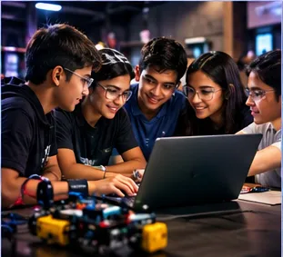
Understanding Artificial Intelligence: Pattern Recognition Labs in Liepaja
Liepaja classes pair model demos with safety rules. Avenvera.com offers broader child development insights. Enquire WhatsApp +92 322 4217059. Supervised platforms only.
AI courses for kids in Liepaja emphasise digital safety and guided practice training image and text classification models on child-safe platforms.
In previous modules, we examined the theoretical foundations of Convolutional Neural Networks (CNNs), including kernel filtering, spatial feature maps, activation functions, and max pooling operations. In this lecture, we translate those theoretical concepts into practical Python code by building an end-to-end image recognition CNN using TensorFlow and Keras.
  ┌─────────────────────────────────────────────────────────────┐
  │              End-to-End Image Recognition Workflow          │
  ├─────────────────────────────────────────────────────────────┤
  │  Step 1: Cloud GPU Environment Setup (Google Colab T4 GPU)  │
  │     • Accelerates tensor processing over standard CPUs      │
  │                                                             │
  │  Step 2: Data Ingestion & Preprocessing (MNIST Dataset)     │
  │     • Load 28×28 grayscale images (10 digit classes)        │
  │     • Normalize pixels (0–255 → 0.0–1.0) & add channel axis │
  │                                                             │
  │  Step 3: CNN Architecture Construction (models.Sequential)  │
  │     • Stack Conv2D, MaxPooling2D, Flatten, and Dense layers │
  │                                                             │
  │  Step 4: Model Parameter Diagnostic (model.summary())       │
  │     • Calculate layer output shapes and 121,930 parameters  │
  │                                                             │
  │  Step 5: Compilation & Training (fit with Adam Optimizer)   │
  │     • Train for 3 epochs with a 10% validation split        │
  │                                                             │
  │  Step 6: Final Evaluation (evaluate on Unseen Test Data)    │
  │     • Measure test loss and test accuracy (98.59%)          │
  └─────────────────────────────────────────────────────────────┘
Cloud Acceleration with Google Colab:
When programming CNNs in Python, training deep networks locally on standard CPUs can be extremely slow. Google Colab provides a free cloud environment equipped with GPU hardware accelerators (such as the T4 GPU).
For this implementation, we utilize the classic MNIST Handwritten Digits Dataset (tf.keras.datasets.mnist), which contains grayscale image samples of handwritten numbers from 0 through 9 across 10 distinct classes.
import tensorflow as tf
from tensorflow.keras import layers, models

# 1. Load the MNIST Dataset
mnist = tf.keras.datasets.mnist
(X_train, y_train), (X_test, y_test) = mnist.load_data()

print(f"Training Images Shape: {X_train.shape}")  # (60000, 28, 28)
print(f"Testing Images Shape : {X_test.shape}")   # (10000, 28, 28)
Pixel Normalization & Channel Axis Expansion:
# 2. Rescale pixel values between 0.0 and 1.0
X_train = X_train / 255.0
X_test = X_test / 255.0

# 3. Add explicit channel axis for grayscale images (28, 28, 1)
X_train = X_train[..., tf.newaxis]
X_test = X_test[..., tf.newaxis]

print(f"Reshaped Train Matrix: {X_train.shape}")  # (60000, 28, 28, 1)
Architectural decisions dictate how effectively a CNN extracts visual features. When designing an architecture, studying established domain research helps save extensive trial-and-error experimentation time.
  ┌─────────────────────────────────────────────────────────────┐
  │                   CNN Layer Architecture                    │
  ├─────────────────────────────────────────────────────────────┤
  │                                                             │
  │   Input Image Layer (28 × 28 × 1 Grayscale)                 │
  │        │                                                    │
  │        ▼                                                    │
  │   Conv2D Layer 1        ──► 32 Filters (3×3), ReLU          │
  │        │                                                    │
  │        ▼                                                    │
  │   MaxPooling2D Layer 1  ──► Pool Size (2×2)                 │
  │        │                                                    │
  │        ▼                                                    │
  │   Conv2D Layer 2        ──► 64 Filters (3×3), ReLU          │
  │        │                                                    │
  │        ▼                                                    │
  │   MaxPooling2D Layer 2  ──► Pool Size (2×2)                 │
  │        │                                                    │
  │        ▼                                                    │
  │   Flatten Layer         ──► Reshapes 2D maps to 1D vector  │
  │        │                                                    │
  │        ▼                                                    │
  │   Dense Hidden Layer    ──► 64 Neurons, ReLU                │
  │        │                                                    │
  │        ▼                                                    │
  │   Output Dense Layer    ──► 10 Neurons, Softmax (Classes)   │
  └─────────────────────────────────────────────────────────────┘
Detailed Layer Breakdown:
# 4. Construct CNN Architecture
model = models.Sequential([
    # First Convolutional Block
    layers.Conv2D(32, (3, 3), activation='relu', input_shape=(28, 28, 1)),
    layers.MaxPooling2D((2, 2)),

    # Second Convolutional Block
    layers.Conv2D(64, (3, 3), activation='relu'),
    layers.MaxPooling2D((2, 2)),

    # Classification Head
    layers.Flatten(),
    layers.Dense(64, activation='relu'),
    layers.Dense(10, activation='softmax')
])
Executing model.summary() displays the complete layer-by-layer spatial shape transformations and trainable parameter counts:
# 5. Print Model Parameter Summary
model.summary()
  ┌─────────────────────────────────────────────────────────────────────────┐
  │                        Model Summary Breakdown                          │
  ├──────────────────────────────┬───────────────────┬──────────────────────┤
  │ Layer (Type)                 │ Output Shape      │ Param #              │
  ├──────────────────────────────┼───────────────────┼──────────────────────┤
  │ conv2d (Conv2D)              │ (None, 26, 26, 32)│ 320                  │
  │ max_pooling2d (MaxPooling2D) │ (None, 13, 13, 32)│ 0                    │
  │ conv2d_1 (Conv2D)            │ (None, 11, 11, 64)│ 18,496               │
  │ max_pooling2d_1 (MaxPooling) │ (None, 5, 5, 64)  │ 0                    │
  │ flatten (Flatten)            │ (None, 1600)      │ 0                    │
  │ dense (Dense)                │ (None, 64)        │ 102,464              │
  │ dense_1 (Dense)              │ (None, 10)        │ 650                  │
  ├──────────────────────────────┴───────────────────┴──────────────────────┤
  │ Total params: 121,930 (476.29 KB)                                       │
  │ Trainable params: 121,930                                               │
  │ Non-trainable params: 0                                                 │
  └─────────────────────────────────────────────────────────────────────────┘
Mathematical Parameter Analysis:
Before training, we compile the model using the Adam optimizer, sparse categorical cross-entropy loss, and the accuracy metric:
# 6. Compile Model Configuration
model.compile(
    optimizer='adam',
    loss='sparse_categorical_crossentropy',
    metrics=['accuracy']
)

# 7. Train Model for 3 Epochs with 10% Validation Split
history = model.fit(
    X_train, y_train,
    epochs=3,
    validation_split=0.1
)
  ┌─────────────────────────────────────────────────────────────┐
  │                 Epoch Training Metrics Log                  │
  ├─────────────────────────────────────────────────────────────┤
  │  Epoch 1/3:                                                 │
  │    • Training Loss: 0.3300  | Training Accuracy: 89.00%     │
  │    • Validation Loss: 0.0500| Validation Accuracy: 98.00%   │
  │                                                             │
  │  Epoch 2/3:                                                 │
  │    • Training Accuracy: 98.00%                              │
  │                                                             │
  │  Epoch 3/3:                                                 │
  │    • Training Accuracy: 98.97% | Training Loss: ~0.0300     │
  │    • Validation Accuracy: 98.65%| Validation Loss: ~0.0400   │
  └─────────────────────────────────────────────────────────────┘
Epoch Training Dynamics:
Finally, we evaluate model generalization on the completely separate test dataset of 10,000 unseen images using model.evaluate():
# 8. Evaluate Model on Test Dataset
test_loss, test_acc = model.evaluate(X_test, y_test)

print(f"\nTest Dataset Loss    : {test_loss:.4f}")
print(f"Test Dataset Accuracy: {test_acc * 100:.2f}%")  # Output: 98.59%
  ┌─────────────────────────────────────────────────────────────┐
  │                   Final Model Performance                   │
  ├─────────────────────────────────────────────────────────────┤
  │  • Test Dataset Loss    : 0.0420                            │
  │  • Test Dataset Accuracy: 98.59%                            │
  │                                                             │
  │  Industry Context:                                          │
  │    • MNIST is a relatively clean benchmark dataset.         │
  │    • Complex client real-world images present higher noise. │
  │    • In production settings, an accuracy around 80% is      │
  │      frequently considered an acceptable baseline.          │
  └─────────────────────────────────────────────────────────────┘
Performance Takeaways:
| Pipeline Stage | TensorFlow / Keras Code | Operational Function | Output Result / Metric |
|---|---|---|---|
| GPU Acceleration | Colab T4 GPU Setup | Enables parallel tensor training. | Accelerated training execution. |
| Data Ingestion | mnist.load_data() | Loads 60k train & 10k test grayscale images. | Array shapes (60000, 28, 28). |
| Preprocessing | X / 255.0 & tf.newaxis | Normalizes pixels to 0–1 & adds channel axis. | Matrix shape (60000, 28, 28, 1). |
| Feature Extractor | Conv2D & MaxPooling2D | Extracts primitive and complex features. | Feature shapes shrink spatially. |
| Classifier Head | Flatten → Dense | Maps 1D feature vector to 10 digit classes. | 10 Softmax output probabilities. |
| Model Summary | model.summary() | Calculates parameter weights per layer. | 121,930 total parameters (~476 KB). |
| Compilation | model.compile() | Sets adam, sparse_categorical_crossentropy. | Configured training pipeline. |
| Training | model.fit() | Trains for 3 epochs with 10% validation split. | Train Acc: 98.97%, Val Acc: 98.65%. |
| Evaluation | model.evaluate() | Evaluates model on 10,000 unseen test images. | 98.59% Test Accuracy. |
Pixel Value Normalization: Raw image pixel intensities range from 0 to 255 based on 8-bit byte representation. To accelerate training convergence, pixel values in both training and testing datasets are normalized by dividing by 255.0 (x_train / 255.0 and x_test / 255.0), scaling all pixel values into a range between 0.0 and 1.0.
Channel Dimension Expansion: CNN layers in Keras expect a 3D input shape (Height, Width, Channels) for each image. Because grayscale datasets like MNIST lack explicit color channels, an explicit channel dimension is added using tf.newaxis to expand the data dimensions to (28, 28, 1).
Hardware Acceleration: Training is typically configured on cloud platforms like Google Colab using a T4 GPU, which substantially speeds up execution compared to standard CPU processing.
The model is built using Keras's Sequential API (tf.keras.models.Sequential) with the following layer stack:
Compilation Settings: The model is compiled using the Adam optimizer, Sparse Categorical Cross-Entropy (sparse_categorical_crossentropy) as the loss function, and Accuracy as the performance metric.
Training Process: The model is trained using model.fit() over 3 epochs with a 10% validation split (validation_split=0.1). Across three epochs, training accuracy increases from ~89% to ~98.97%, while validation accuracy reaches ~98.65%.
Model Evaluation & Results: Evaluating the trained model on the unseen test dataset via model.evaluate() achieves a high test accuracy of 98.59%.
ChatGPT for Kids on Udemy.
Disclosure: This page contains affiliate links. We may earn from qualifying purchases at no extra cost to you. Links are intended for parents and educators, not as marketing directed at young children.
Liepaja classes pair model demos with safety rules. Avenvera.com offers broader child development insights. Enquire WhatsApp +92 322 4217059. Supervised platforms only.
Students learn to protect personal data, avoid sharing private details online, and evaluate AI output critically.
Students train image and text classification models using guided, child-safe platforms.
Insights on child growth and learning are available at Avenvera.com.